This is part two of a three-part series on Exascale. If you haven’t read the first part, I recommend checking it out here.

---

Exascale Software

---

As Exascale comes to replace ASM as an integral storage management system on Exadata platforms, it’s expected that its software runs on a specific site. ASM operated as part of the Grid Infrastructure, and in its initial versions, there was one ASM instance per RAC node, since communication between ASM instances and local database instances occurred via IPC protocol. In the more recent architecture of ASM flex, communication between ASM instances and databases already used “Oracle Net Services,” allowing an ASM instance to handle requests from local databases or other RAC nodes. However, it was still necessary to have multiple ASM instances spread across nodes to ensure the high availability of this service.

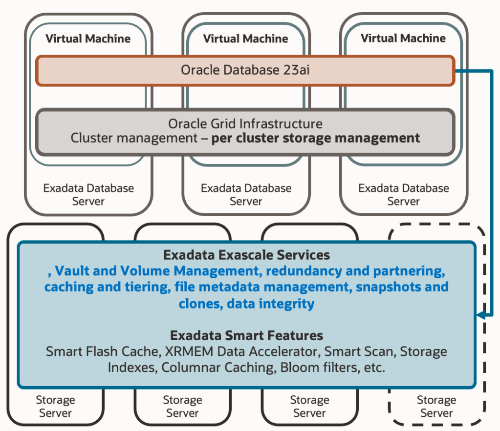
The first change introduced by Exascale architecture is that Exascale software has moved to Exadata’s storage cells. Those of you with experience in Exadata probably know this software from interacting with it locally in the cells through the “cellcli” binary. We use this binary to fetch specific metrics, define IORM plans, set certain behavioural parameters, and other tasks. It is this Exadata software that performs all the magic behind the scenes, moving hot objects between different storage tiers (hard disk, flash cache, RAM), maintaining in-cell indexes, ensuring IO quality of service for each entity, and much more.

This means we now have the service previously provided by ASM redundantly as many times as there are cells in the Exadata system. Additionally, there’s no need to install and maintain ASM software on compute nodes, and the effort developed by Exascale software is spread among more participants. Although you might see satellite Exascale processes on compute nodes, the bulk of the work is offloaded to the storage cell software:

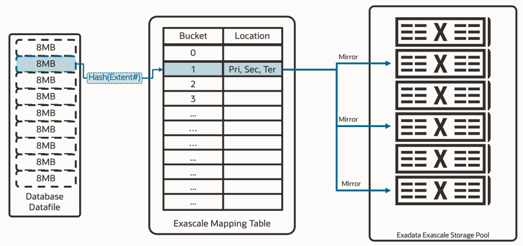
Exascale continues to be an extent mapper, to avoid creating intermediate layers between the database and storage. This means it still requires a mapping structure where each extent is uniquely related to the physical address that contains the data. The following diagram shows this concept, where we already see a change; extents have increased in size to 8MB, as a balance point to provide good performance without reducing the granularity of data distribution across different griddisks.

---

Exascale Internals

---

But that diagram, that architecture, would not be enough to overcome the limitations we previously discussed about ASM. Exascale introduces a crucial intermediary component between the extents and the physical data locations called the “Exascale Mapping Table.” This table contains two columns: a column for buckets and a column for physical locations. The extents now relate to the buckets, but it’s not necessarily a 1-1 relationship. It’s possible that two extents from two different databases point to the same bucket; this will occur if we perform a “thin clone” (aka. snapshot clone, snapshot copy). Then, that bucket will contain the physical location of the content of that bucket (of that extent or those extents). But not just one physical location, rather the location of all copies of that extent. This means we have the capability to define data redundancy at the extent level.

With this key piece called “mapping table,” which is native to Oracle’s own software, we have solved the problem of both “thin clones” and different levels of data redundancy. In more detail:

Solution to thin clones: Previous strategies of using a SPARSE DISKGROUP or an FS ACFS (or even NFS or others) resolved thin clones by delegating the capability to the storage layer. That is, for ASM, one extent pointed to a physical address, and another extent (from a thin clone) pointed to a different physical address. But the storage layer knew one was a thin clone of the other, ensuring both ended up accessing the same data. Exascale now understands and manages these relationships natively, which allows for a far superior integration with the rest of the capabilities.

Solution to different levels of data redundancy: With a standard ASM diskgroup, we could choose redundancy for all the content of the same diskgroup. With ASM flex, we could choose redundancy for groups within the same diskgroup. Exascale now has the capability to determine redundancy down to the extent level, achieving the highest possible flexibility.

The mapping table is managed autonomously in all cases, and it isn’t continuously accessed by the databases. The system is designed so that each database has a cached copy of the mapping table to reduce latency and load to the maximum. If the location of the data has changed, the cells will automatically reject the IO and send the refreshed table to the database instances so they can continue working.

---

Storage Structures

---

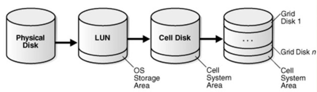
But there’s still more to address. How do we solve the problem of space compartmentalization, which occurs in environments with several Virtual Clusters? The solution involves redesigning the original approach of ASM storage entities in Exadata. That architecture where we created Celldisks from partitions of physical disks, and Griddisks using portions of Celldisks. We finally created DISKGROUPS using Griddisks from different storage cells (failgroups). Diskgroups that were only visible to a specific Virtual Cluster.

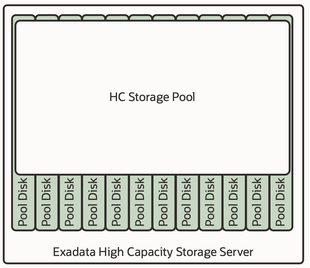
Would it be possible to create a “Diskgroup” accessible by any database, and from any Virtual Cluster within the same infrastructure? This approach is what Exascale is aimed at. In an architecture paradoxically simpler than before, we now create the new entity “Pool Disks” from the system disks, and with them, we create a “Storage Pool.” A storage space that:

• Is accessible from any Virtual Cluster, thus, a structure that eliminates space compartmentalization in cell among Virtual Clusters. A pool for all VCs.
• A storage that can store any type of information, whether “DATA” or “RECO”.
• A storage that works with the mapping table, and that offers any type of redundancy (defined at the file type level) and with native thin cloning capability (in its same location).

If you’re not thrilled by now… well, keep reading.

So, If we have a shared storage pool, what remains to be addressed to complete the solution? Create logical containers within the pool that allow us to group – if we want – several databases from the same or different VC :

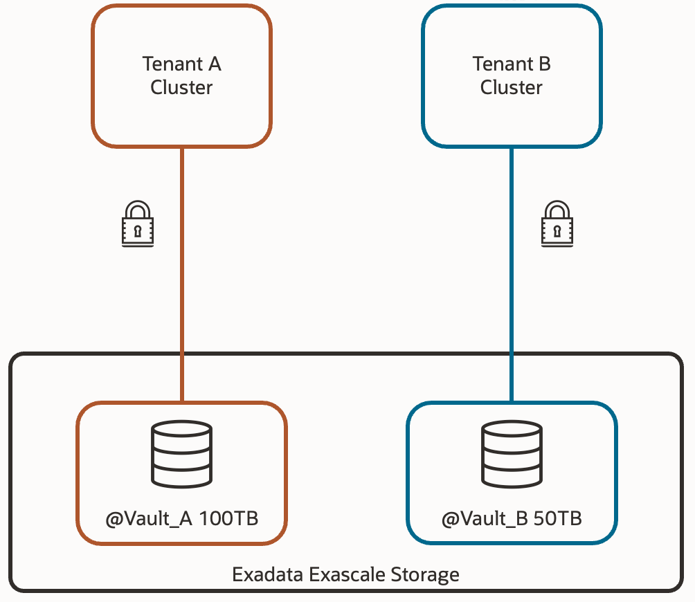
These structures are called Vaults, and they are what really come to replace the diskgroups from the database perspective. That is, within the database, instead of using +DATA, we’ll use @vault_prod1 – for example. We’ll be able to define a maximum storage space for each pool, so that certain databases don’t consume space that others might need. Additionally, we can associate IORM policies for each of the vaults, including maximum IOPS, usable flash cache size, usable XRMEM size, and usable Flash Log space.

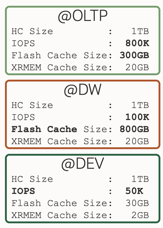
This way, we have the option to differentiate the storage qualitatively between productive and non-productive databases. Or transactional databases from informational databases; each one with resources adjusted to their nature.

---

Up Next: Exadata Database Service on Exascale Infrastructure

---

I hope you find this new architecture as interesting as I do. In the next article, I’ll explain how Oracle has used this new approach to create a new service in OCI called “Exadata Database Service on Exascale Infrastructure”.

If you want to delve into more detail, I recommend accessing Oracle’s official Exascale documentation, where you’ll see other interesting concepts like storage rings, which will help you understand in more detail how redundancy is maintained, among other interesting topics.

See you in the next post about Exadata Database Service on Exascale Infrastructure!